【선형대수학】 선형대수학 문제 [01-20]
선형대수학 문제 [01-20]
추천글 : 【선형대수학】 선형대수학 목차
문제 1. Solve the following linear system:

The given problem is as follows:

Thus, the augmented matrix is as follows:

When running the following Python code:
A = Matrix([[1,2,1,1],[3,6,2,2],[1,2,1,2]])
A_rref = A.rref()
A_rref[0]
I met the following:

The last row of the RREF doesn't hold true.
Thus, the linear system is inconsistent.
That is, there is no solution to this linear system.
문제 2. Solve the following linear system:

The given problem is as follows:

Thus, the augmented matrix is as follows:

When running the following Python code:
A = Matrix([[2,4,1,4],[1,2,1,3],[1,2,0,1]])
A_rref = A.rref()
A_rref[0]
I met the following:

Thus, the number of the solution of this linear system is infinite as follows:

문제 3. Solve the following linear system:

The given problem is as follows:

Thus, the augmented matrix is as follows:

When running the following Python code:
A = Matrix([[2,2,5,4],[1,-1,-1,-1],[1,-1,1,1]])
A_rref = A.rref()
A_rref[0]
I met the following:

Thus, the solution of the linear system is only one as follows:

문제 4. Consider the following vectors:

⑴ Are the vectors {u1, u2, u3} linearly independent?
To identify the linear independence of the three vectors, we need to consider the following:

Thus, the augmented matrix is as follows:

When running the following Python code:
A = Matrix([[2,-4,-1,0],[4,-8,-1,0],[6,-12,-6,0],[1,-2,-6,0],[0,0,6,0]])
A_rref = A.rref()
A_rref[0]
I met the following:

Thus, u1, u2, and u3 are not linearly independent, as c1, c2, and c3 are necessarily zeros.
For example, c1 = 2, c2 = 1, c3 = 0 can satisfy the above linear system. That is,

⑵ Is the vector u4 in the span of {u1, u2, u3}?
To identify whether the vector u4 is the span of {u1, u2, u3}, we need to consider the following:

Thus, the augmented matrix is as follows:

When running the following Python code:
A = Matrix([[2,-4,-1,3],[4,-8,-1,7],[6,-12,-6,6],[1,-2,-6,-4],[0,0,6,6]])
A_rref = A.rref()
A_rref[0]
I met the following:

For example, c1 = 0, c2 = -1, c3 = 1 satisfies the above linear system. That is,

The existence of the solutions implies that the vector u4 is the span of {u1, u2, u3}.
문제 5. Let V = span{u1, u2, u3, u4, u5}, with

⑴ Find a basis for V and explain why it is a basis.
Solution 1
Basis refers to a set of linearly independent vectors that span a space.
Firstly, u1, u2, u3, u4, and u5 are not linearly independent due to the following:

Secondly, u3 and u5 can be expressed with u1, u2, and u4 according to the following:

Thus, one of the bases of V is {u1, u2, u4}.

Solution 2
Note that the 4th and 5th elements of each vector match the 1st and 2nd elements respectively, implying:

The determinant from the first three rows from u1, u2, and u4 is not zero as follows:

Thus, u1, u2, and u4 are linearly independent and span the image of V.
Therefore, {u1, u2, u4} is a basis for V.
⑵ Extend the basis of V to a basis of ℝ5; i.e., find a basis of ℝ5 that includes the basis of V. (Hint: try adding the standard basis of ℝ5 to the basis of V.)
Solution 1
Let's reverse RREF process to extend the basis of V to span ℝ5.

Thus, {u1, u2, u4, e4, e5} spans ℝ5.
Solution 2

Thus, {u1, u2, u4, e4, e5} spans ℝ5.
문제 6. Let W be the set of common solutions to the following equations:

Find a basis for W and explain why it is a basis.
Let's think of the following linear system:

When running the following Python code:
A = Matrix([[1,1,3,2,-1],[3,0,3,3,3],[1,1,3,2,-1]])
A_rref = A.rref()
A_rref[0]
I met the following:

Thus, each element of W can be expressed as follows:

It is evident that (-1, -2, 1, 0, 0)T, (-1, -1, 0, 1, 0)T, (-1, 2, 0, 0, 1)T are linearly independent, when examining the numbers in blue. Therefore, {(-1, -2, 1, 0, 0)T, (-1, -1, 0, 1, 0)T, (-1, 2, 0, 0, 1)T} forms a basis because they are linearly independent and span the solution space W.
문제 7. Let T : ℝ3 → ℝ2 be a linear transformation sending the vector (1, 1, -1)T to the vector (0, 0)T, and the vector (1, -1, 1)T to the vector (1, 2)T.
⑴ Find T(z), where z = (1, 5, -5)T. (Hint: use the fact that T is linear.)

⑵ There are infinitely many such linear transformations T satisfying the above requirements; find all their matrices, and check they satisfy the constraints above.
Solution 1

Therefore, there are infinitely many such linear transformations T that satisfy the given requirements.
Solution 2

문제 8. Find a basis 𝔅 of ℝ2 such that

What is the matrix of the linear transformation that maps a vector in standard coordinates to a vector in new coordinates?
Let A be the matrix corresponding to the linear transformation that maps a vector in standard coordinates to a vector in new coordinates.

A-1 transforms bases e1’, e2’ in the new coordinates to (2, -1)T, (2, 2)T in standard coordinates, respectively.
Note that e1 and e2 are bases for the standard cartesian coordinates while e1’ and e2’ are bases for the new coordinates.
문제 9. Find a basis 𝔅 for the plane x1 + 2x2 + x3 = 0 (a plane in ℝ3), such that the vector v = (1, -1, 1)T has coordinates [v]𝔅 = (2, -1)T with respect to this basis.
Solution 1
Let A be the matrix corresponding to the linear transformation that maps a vector in standard coordinates to a vector in new coordinates.

Let a = 1, b = -1, c = d = e = 0, f = -1, as this problem only requires an example solution.
Note that there is no unique answer but an infinite number of answers.
Let’s find what vectors are transformed to e1’ and e2' when they are the bases for the new coordinates.

Also,

Alternatively, the validation of my answer can be fulfilled with v = (1, -1, 1)T, [v]𝔅 =(2, -1) as follows:

Solution 2 (ref)
Let B = {w1, w2} be the basis of the given plane x1 + 2x2 + x3 = 0 (a plane in ℝ3).
Then any v in the plane can be uniquely written as:

where c1 and c2 are the 𝔅-coordinates of x, i.e.

Therefore,

If w1 be any vector in the plane x1 + 2x2 + x3 = 0, w2 = 2w1 – v.
If w1 is not parallel to v, w1 and w2 are linearly independent.
Also, as w1 and w2 are on the plane, they span the whole plane.
Thus, the basis of this plane is {w1, 2w1 - v}.
In the above example, I found:

문제 10. Consider the matrix
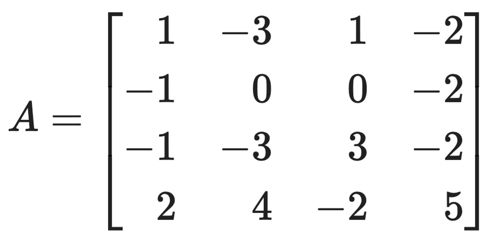
⑴ Find the characteristic polynomial of A.

The Python code is as follows:
import sympy as sp
x = sp.symbols('x')
matrix = sp.Matrix([
    [1 - x, -3, 1, -2],
    [-1, -x, 0, -2],
    [-1, -3, 3 - x, -2],
    [2, 4, -2, 5 - x]
])
determinant = matrix.det()
determinant
Then, I met x4 - 9x3 + 29x2 - 39x + 18.
⑵ Find the eigenvalues of A and check that they are roots of the characteristic polynomial.
When running the following Python code:
from sympy import *
A = Matrix([
    [1, -3, 1, -2],
    [-1, 0, 0, -2],
    [-1, -3, 3, -2],
    [2, 4, -2, 5]
])
eigenvalues = A.eigenvals()
eigenvalues
I met the following:
{2: 1, 1: 1, 3: 2}
It means that λ=1 and λ=2 have a multiplicity of one, while λ=3 has a multiplicity of two.
Consistently, we can check they are roots of the characteristic polynomial as follows:

⑶ Find all eigenvalues of A using the definition of eigenspace as a nullspace of a suitable matrix (you can use Python's rref), and compare your answer using Python's np.linalg.eig. How are they related?
Solution 1
For λ=1, I need to consider the following equation and the corresponding augmented matrix:

When running the following Python code:
A = Matrix([
    [1-1, -3, 1, -2, 0],
    [-1, 0-1, 0, -2, 0],
    [-1, -3, 3-1, -2, 0],
    [2, 4, -2, 5-1, 0]
])
A_rref = A.rref()
A_rref[0]
I met the following:

Let's consider x1 + x4 = 0, x2 + x4 = 0, x3 + x4 = 0 to satisfy the above linear system.
Thus, eigenvector corresponding to λ=1 is (-1, -1, -1, 1)T.
Similarly, the eigenvector corresponding to λ=2 is (-1, -1/2, -1/2, 1)T.
Lastly, the eigenvector corresponding to λ=3 is (-1/2, -1/2, -1/2, 1)T.
Let's check the following

The above calculation is based on the definition of eigenspace as a nullspace of a suitable matrix.
Meanwhile, to acquire eigenvectors from np.linalg.eig, I ran the following Python code.
import numpy as np
A_np = np.array([
    [1, -3, 1, -2],
    [-1, 0, 0, -2],
    [-1, -3, 3, -2],
    [2, 4, -2, 5]
])
eigenvalues_np, eigenvectors_np = np.linalg.eig(A_np)
print(eigenvalues_np)
print(eigenvectors_np)
I met the following:
[2.+0.00000000e+00j 3.+2.71847221e-08j 3.-2.71847221e-08j
1.+0.00000000e+00j]
[[ 0.63245553+0.00000000e+00j -0.37796447-5.13742958e-09j
-0.37796447+5.13742958e-09j 0.5 +0.00000000e+00j]
[ 0.31622777+0.00000000e+00j -0.37796447+5.13742958e-09j
-0.37796447-5.13742958e-09j 0.5 +0.00000000e+00j]
[ 0.31622777+0.00000000e+00j -0.37796447-5.13742958e-09j
-0.37796447+5.13742958e-09j 0.5 +0.00000000e+00j]
[-0.63245553+0.00000000e+00j 0.75592895+0.00000000e+00j
0.75592895-0.00000000e+00j -0.5 +0.00000000e+00j]]
Two eigenvectors (■, ■) from λ=3 are identical as the imaginary parts of them are almost zero.
An extra eigenvector appears in np.linalg.eig because of rounding errors.
The above calculation is based on Python's np.linalg.eig.
Solution 2
Note that the algebraic multiplicity of λ=3 is two and the geometric multiplicity of it is one.
In this case, there is a vector satisfying:

This vector is called a generalized eigenvector.
⑷ Is A diagonalizable? If so, find a change of coordinates that puts A in diagonal form; if not, explain why.
When a matrix X of size n × n is diagonalizable, it means the following:
X = PDP-1
where D is a diagonal matrix and P is a matrix of eigenvectors.
The existence of the inverse matrix of P implies X has n linearly independent eigenvectors.
As the number of eigenvectors of A is only three (< 4), A is not diagonalizable.
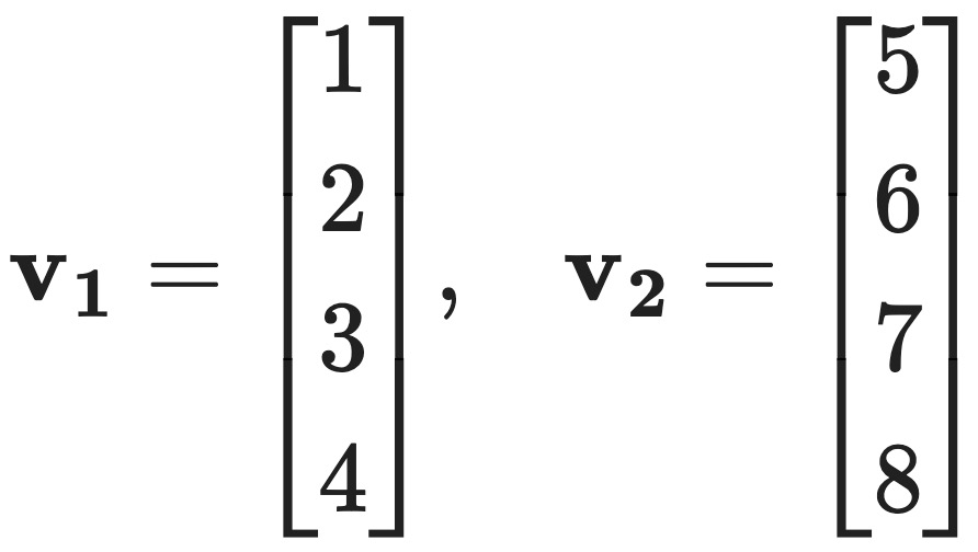
문제 11. For a subspace V of ℝn, the orthogonal complement V⊥ of V is the set of vectors in ℝn that are orthogonal to all vectors in V. Note that V⊥ is a subspace of ℝn. Find a basis for V⊥, where V = span{v1, v2}, with
Solution 1
I’ve just come up with (1, 1, 2, 2)T and (1, 3, 3, 1)T in addition to v1 and v2.
Let’s check {v1, v2, (1, 1, 2, 2)T, (1, 3, 3, 1)T} spans ℝ4 as follows:

Now, let’s describe the Gram-Schmidt orthogonalization process, a method to obtain an orthogonal basis from an arbitrary basis; note that ⟨·, ·⟩ means dot-product.

Let’s check ⟨yi, yj⟩i≠j = 0.
Thus, I could find a basis {y3, y4} for V⊥.
Solution 2
Let’s normalize y1 and y2 as follows:

Let’s consider the transformation that projects an arbitrary vector onto the plane spanned by the orthonormal basis as follows:
UUT = u1u1T + u2u2T
I ran the following Python code:
y1 = np.array([1, 2, 3, 4])
y2 = np.array([8/3, 4/3, 0, -4/3])
u1 = y1 / np.linalg.norm(y1)
u2 = y2 / np.linalg.norm(y2)
U = np.column_stack((u1, u2))
UUT = np.dot(U, U.T)
v1 = np.array([1, 1, 2, 2])
v2 = np.array([1, 3, 3, 1])
proj_v1 = np.dot(UUT, v1)
proj_v2 = np.dot(UUT, v2)
proj_v1, proj_v2
Thus, (1, 1, 2, 2)T and (1, 3, 3, 1)T can be transformed to (0.9, 1.3, 1.7, 2.1)T, (2, 2, 2, 2)T.
Therefore, two vertical vectors to the image of span{v1, v2} are the following, respectively:

문제 12. Let u1, u2, u3, u4, u5 be orthonormal vectors in ℝ8.
⑴ Find the length of the vector v = 2u1 - u2 - u3 + 3u5.

⑵ Find the angle between the vectors v = 2u1 - u2 - u3 + 3u5 and w = u1 + u2 + u3 - u4.

Thus, v and w are perpendicular (= 90°) to each other.
⑶ For a vector x ∈ ℝ8, what is the relationship between (xTu1)2 + (xTu2)2 and ||x||2? When are these two quantities equal?
We can represent x as (x1, x2, x3, x4, x5, x6, x7, x8)T.
Thus, the following relationship holds:

문제 13. Solve the following problems.
⑴ Let T be the orthogonal projection in ℝ3 onto the plane x1 + x2 + x3 = 0. Find all the eigenvalues and eigenvectors of T (do not find the matrix of T: think about it geometrically). Hint: 0 = x1 + x2 + x3 = (1, 1, 1)T · (x1, x2, x3)T, which means that the vectors on the plane are precisely the vectors perpendicular to (1, 1, 1)T.
The problem can be visualized as follows.
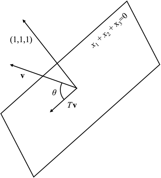
We should calculate λ and v such that Tv = λv.
If θ = 0, Tv always equals to v, indicating λ = 1 and eigenvectors are the basis of the plane.
For example, (1, -1, 0)T, (1, 0, -1)T on the plane can be two eigenvectors corresponding to λ = 1.
If θ = π / 2, Tv always equals to 0, indicating λ = 0 and the eigenvector is (1, 1, 1)T.
Otherwise, Tv ≠ λv by intuition.
⑵ Now let A be the matrix of the orthogonal projection in ℝ3 onto the plane x1 + x2 + x3 = 0.
① Find the matrix A.
Solution 1
We can find (1, -1, 0)T, (1, 0, -1)T - 0.5 (1, -1, 0)T as orthogonal basis for the plane x1 + x2 + x3 = 0.

I ran the following Python code:
y1 = np.array([1, -1, 0])
y2 = np.array([1-0.5, 0.5, -1])
u1 = y1 / np.linalg.norm(y1)
u2 = y2 / np.linalg.norm(y2)
U = np.column_stack((u1, u2))
UUT = np.dot(U, U.T)
UUT
Thus, A is as follows:

Solution 2
Let's think of an arbitrary vector v = (v1, v2, v3)T in ℝ3.
The orthogonal projection of the vector onto the plane x1 + x2 + x3 = 0 is as follows:

Thus, A is as follows:

② Find all the eigenvalues and eigenvectors of A (and check that you answer matches the result of part ⑴ above.
Let’s solve the following characteristic polynomial:

If λ = 2/3, the polynomial can be expressed as follows:

If λ ≠ 2/3, the polynomial can be expressed as follows:

Thus, eigenvalues are λ = 0 and λ = 1.
If λ = 0, the eigenvector is as follows:

If λ = 1, two eigenvectors are as follows:

They match the result of ⑴.
③ Is A diagonalizable? If so, find its diagonal form, and the change of coordinates that diagonalizes A.
Solution 1
n × n matrix A is diagonalizable if and only if A has n linearly independent eigenvectors.
Thus, A is diagonalizable.
Let’s define the diagonal form and the eigenvector matrix as P and D, respectively:

Solution 2

④ Find the point on the plane x1 + x2 + x3 = 0 which is closest to (2, 3, 7)T, and find the distance between the two.
Let’s consider the projection of (2, 3, 7)T to the plane:

The projected point on the plane is the closest to (2, 3, 7)T.
The Euclidean distance between them is as follows:

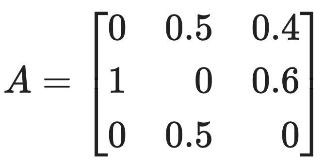
문제 14. Consider the Markov Chain with transition matrix:
⑴ What is the probability that the chain goes from state 3 to state 1 in one step? What is the probability that the chain goes from state 3 to state 1 in exactly 3 steps? What is the probability that the chain goes from state 3 to state 1 in at most 3 steps?
When A is a transition matrix, Aij represents the probability of transitioning from state j to state i.
Thus, the probability that the chain goes from state 3 to state 1 in one step is A13 = 0.4.
Let’s consider A2 and A3 as follows:

Thus, the probability that the chain goes from state 3 to state 1 in exactly 3 steps is A313 = 0.32.
Also, the probability that the chain goes from state 3 to state 1 in at most 3 steps is as follows:

⑵ Is the chain regular? Explain.
A Markov chain is said to be a regular Markov chain if some power of its transition matrix A (i.e., Ak) has only positive entries.
I used the following Python code to calculate A4:
A_sym = Matrix([
    [0, 0.5, 0.4],
    [1, 0, 0.6],
    [0, 0.5, 0]
])
A_sym_4 = A_sym**4
A_sym_4
As a result, I met the following:

Thus, the existence of Ak having all positive entries implies A is regular.
⑶ How many equilibrium solutions does the chain have?
Being “strongly connected” refers to a state in which, for any node i in the graph, it is possible to reach any other node j; meanwhile, being “regular” means that for some natural number k, all elements of Mk are positive (i.e., non-zero).
Therefore, if a matrix is regular, it implies that it is strongly connected, but the reverse does not necessarily hold.
regular ⊂ strongly connected
Thus, the matrix A is strongly connected as verified in Problem ⑵.
According to Perron-Frobenius theorem, if the transition matrix P is a strongly connected matrix, there exists a stationary distribution vector of state q subject to:
Pq = q
Thus, the matrix A has only one equilibrium solution.
⑷ Find the limit as t goes to infinity of At.

The period of a specific node i is the greatest common divisor of all the paths leading from node i back to itself; thus, the period of each node is 1.
According to the Perron-Frobenius theorem, as transitioin matrix in a Markov chain A is strongly connected and aperiodic, Akij converges to qi as k goes to infinity, which implies that for any fixed i, the value converges to the same result regardless of j.
Thus, A∞ can be expressed as follows:

⑸ Consider the vector x0 = (0.3, 0.3, 0.4)T. Find the limit as t goes to infinity of Atx0.
The equilibrium state x∞ is q regardless of the initial state x0 as follows:

문제 15. Consider the matrix:
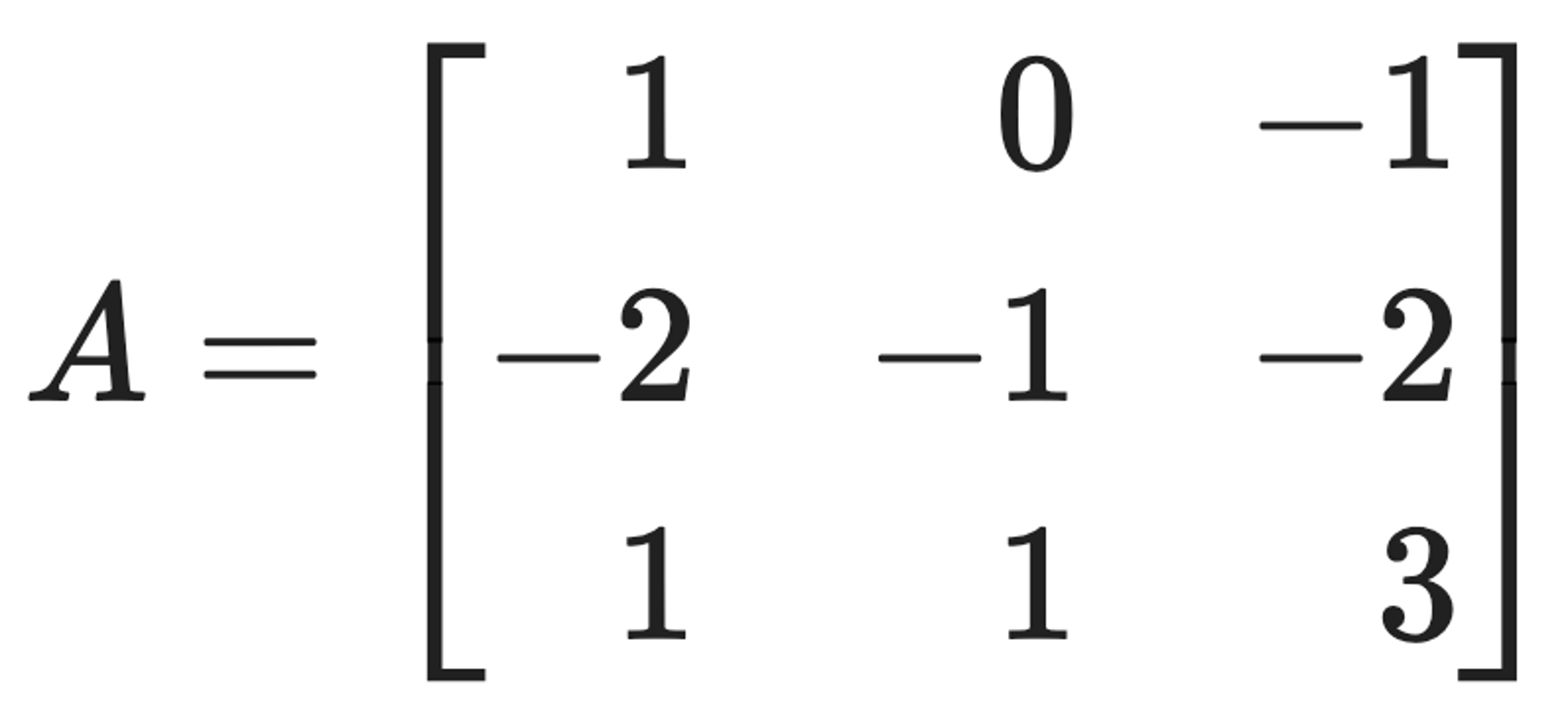
and the vector x0 = (2, 0, 0)T. Find closed formulas for Atx0, that is, write Atx0 as (f(t), g(t), h(t)) for some explicit functions f(t), g(t), h(t).
I could find the generalized form of At as follows:

I can see the above satisfies when t = 1.
If the above form holds for k = 1, ···, t, I can confirm that At+1 also follows the same form:

Thus, the generalized form of At holds by mathematical induction.
Therefore, I get

문제 16. In this problem, do not use any Python function to find least square solutions such as np.linalg.lstsq, but only basic matrix algebra.
⑴ Find the function of the form f(x) = c0 + c1 sin(x) + c2 cos(x) + c3 sin(2x) + c4 cos (2x) that best fits the data points (0, 0), (0.5, 0.5), (1, 1), (1.5, 1.5), (2, 2), (2.5, 2.5), (3, 3), using least squares. What is the predicted value of this model for the point x = 1.7?
Solution 1

The predicted value of the model for the point x = 1.7 is as follows:
1.5 + 0.1090 sin(1.7) - 1.5367 cos(1.7) + 0.3027 sin(3.4) + 0.0431 cos(3.4) = 1.6871 ≅ 1.7
Solution 2

Thus, I ran the following Python code:
import numpy as np
t_data = np.array([0, 0.5, 1, 1.5, 2, 2.5, 3])
y_data = np.array([0, 0.5, 1, 1.5, 2, 2.5, 3])
A = np.column_stack([
    np.ones(len(t_data)),            # c0
    np.sin(t_data),                  # c1 (sin(t))
    np.cos(t_data),                  # c2 (cos(t))
    np.sin(2*t_data),                # c3 (sin(2t))
    np.cos(2*t_data)                 # c4 (cos(2t))
])
coeffs = np.linalg.inv(A.T @ A) @ A.T @ y_data
coeffs
As a result, I met
array([ 1.5 , 0.10897422, -1.53669122, 0.30269197, 0.04314769])
⑵ Repeat ⑴ using Ridge regression with λ = 0.1. Remember to standardize the data and that the model on standardized data has no constant term.

If each feature has different scale, a certain feature can affect the regression significantly.
Features with larger values tend to have larger coefficients, leading to stronger regularization, which can cause the coefficients to become excessively small.
On the other hand, features with smaller values tend to have smaller coefficients and may be under-regularized, resulting in insufficient regularization.
That’s why the standardization is needed when conducting panelized regression.
I ran the following Python code to conduct feature-wise standardization and acquire the coefficients:
import numpy as np
t_data = np.array([0, 0.5, 1, 1.5, 2, 2.5, 3])
y_data = np.array([0, 0.5, 1, 1.5, 2, 2.5, 3])
A = np.column_stack([
    np.sin(t_data),                  # c1 (sin(t))
    np.cos(t_data),                  # c2 (cos(t))
    np.sin(2*t_data),                # c3 (sin(2t))
    np.cos(2*t_data)                 # c4 (cos(2t))
])
A_mean = np.mean(A, axis=0)
A_std = np.std(A, axis=0)
A_standardized = (A - A_mean) / A_std
lambda_ridge = 0.1
I = np.eye(A_standardized.shape[1])
ridge_coeffs = np.linalg.inv(A_standardized.T @ A_standardized + lambda_ridge * I) @ A_standardized.T @ y_data
ridge_coeffs
As a result, I could acquire the following:

To predict a certain value, we need to bring the constant c0 = 1.5 from Problem ⑴.
Thus, the predicted value of the model for the point x = 1.7 is 1.6922 with the following code:
t_new = 1.7
A_new = np.array([
    np.sin(t_new),                  # c1 (sin(t))
    np.cos(t_new),                  # c2 (cos(t))
    np.sin(2 * t_new),              # c3 (sin(2t))
    np.cos(2 * t_new)               # c4 (cos(2t))
])
A_new_standardized = (A_new - A_mean) / A_std
prediction = A_new_standardized @ ridge_coeffs
prediction + 1.5
문제 17. Consider the matrix:

⑴ Find all singular values of A (including the zero ones, if any) using the definition of singular values.
Solution 1
I ran the following Python code:
import numpy as np
A = np.array([[0,1,1,-1],
            [1,1,0,-1]])
U, s, Vt=np.linalg.svd(A)
print(U)
print(s)
print(Vt)
Then, I get
[[ 0.70710678 -0.70710678]
 [ 0.70710678  0.70710678]]
[2.23606798 1.        ]
[[ 3.16227766e-01  6.32455532e-01  3.16227766e-01 -6.32455532e-01]
 [ 7.07106781e-01 -3.59307145e-17 -7.07106781e-01  8.17513888e-18]
 [ 5.18306027e-01 -6.64367251e-01  5.18306027e-01 -1.46061224e-01]
 [ 3.62434632e-01  3.98266438e-01  3.62434632e-01  7.60701071e-01]]
Therefore, the non-zero singular values of A are σ1 = √5 and σ2 = 1, with σ3 = σ4 = 0 representing the two zero singular values.
Note that there are two singular values, considering that the matrix is a 2 × 4 matrix, as follows:

Also note that the number of non-zero singular values of A is rank(A).
Solution 2

The singular values of A are eigenvalues of AAT as follows:

Similarly, ATA can also be used to calculate singular values.

⑵ Write SVD of A.
Solution 1

Note that SVD is not uniquely determined. For example, there is another example as follows:

Solution 2

⑶ Find the best rank 1 approximation of A.
To find the best rank-k approximation of A, one should eliminate the smallest singular values σr, σ(r-1), ⋯ from A = UΣVT = σ1 u1 v1T + ⋯ + σr ur vrT, σ1 ≥ ⋯ ≥ σr.
Thus, the best rank 1 approximation of A is as follows:

Alternatively, the explicit matrix can be represented as:

문제 18. Consider the quadratic form

⑴ Find a matrix A such that f(x) = xTAx.
Quadratic form can be represented as follows:

Thus, the matrix A ∈ R4×4 should be as follows:

⑵ Find the maximum value and all points of maximum value of f under the constraint ||x|| = 1.
The following holds under the constraint of ‖x‖ = 1:

To calculate eigenvalues and eigenvectors, I ran the following Python code:
import numpy as np
a = np.array([
    [1, 1, 3, 0],
    [1, -1, 1, 4],
    [3, 1, 3, 0],
    [0, 4, 0, 5]
])
eigenvalues, eigenvectors = np.linalg.eig(a)
print("Eigenvalues:", eigenvalues)
print("Eigenvectors:")
print(eigenvectors)
As a result, I met the following:
Eigenvalues: [ 7.2073836   5.14374872 -1.14374872 -3.2073836 ]
Eigenvectors:
[[ 0.19319274  0.54808834  0.79673917 -0.16577824]
 [ 0.45881421 -0.01245022  0.0813939   0.88470874]
 [ 0.24680241  0.76119687 -0.59646749 -0.06240536]
 [ 0.83141726 -0.34644406 -0.05299299 -0.43117699]]
Thus, the maximum value is λ1 = 7.2073836 and the corresponding point of maximum value is:

문제 19. Find all critical points of the function

and use the second derivative test to classify them.
The gradient of f is as follows:

Thus, the critical point(s) should satisfy the following conditions:

Therefore, the critical points are (1,0,0,0) and (-1,0,0,0).
Hessian matrix is as follows:

For (1,0,0,0), the characteristic polynomial of

are (2 - λ){(2 - λ)2(-λ) - (2 - λ)} = (2 - λ)2 {λ2 - 2λ - 1}. Thus, three eigenvalues are positive, and the other one is negative, making Hf indefinite matrix and (1,0,0,0) saddle point.
For (-1,0,0,0), the characteristic polynomial of

are (-2 - λ){(-2 - λ)(2 - λ)(-λ) - (2 - λ)} = (-2 - λ)(2 - λ){λ2 + 2λ - 1}. Thus, two eigenvalues are positive, and the other two are negative, making Hf indefinite matrix and (-1,0,0,0) saddle point.
문제 20. In this problem, do not use any Python function to perform PCA, but only linear algebra. Consider the following five data points:

⑴ Find the directions of the first two principal components using the covariance matrix.
Solution 1

Since the given sample represents the entire population, the population mean is known, so the sample covariance matrix C is calculated by dividing by n instead of n−1.
The eigenvalues of C are 84.56, 13.95, 2.527, and 0.005.
The first two highest eigenvalues of C are 84.56 and 13.95, and their corresponding eigenvectors are:

Solution 2
To implement the problem with Python code, one can run the following:
import numpy as np

# Define the centered matrix
Xc = np.array([
    [-0.2, -2.0, 0.4, 1.4],
    [-1.2, -2.0, 1.4, -2.6],
    [1.8, -1.0, 0.4, 7.4],
    [-3.2, -6.0, -7.6, -11.6],
    [2.8, 11.0, 5.4, 5.4]
])

# Compute (1/5) * Xc^T * Xc
C = (1 / 5) * Xc.T @ Xc

# Display the result
print(C)

# Calculate eigenvalues and eigenvectors from sample covariance matrix
matrix = C
eigenvalues, eigenvectors = np.linalg.eigh(matrix)
sorted_indices = np.argsort(eigenvalues)[::-1]
sorted_eigenvalues = eigenvalues[sorted_indices]
sorted_eigenvectors = eigenvectors[:, sorted_indices]
print("Eigenvalues:\n", sorted_eigenvalues)
print("\nEigenvectors:\n", sorted_eigenvectors)
Then, I get
[[ 4.56 10.2   7.68 13.68]
 [10.2  33.2  20.2  24.8 ]
 [ 7.68 20.2  17.84 23.44]
 [13.68 24.8  23.44 45.44]]
Eigenvalues:
 [8.45608028e+01 1.39476448e+01 2.52654218e+00 5.01026794e-03]

Eigenvectors:
 [[-0.22753049  0.04518928 -0.24313071  0.94184673]
 [-0.54435705 -0.75127681 -0.32696734 -0.17986363]
 [-0.43088204 -0.10485083  0.88683763  0.12986911]
 [-0.68282205  0.65003645 -0.21794226 -0.25240409]]
⑵ Find the directions of the first two principal components using the Singular Value Decomposition.
Solution 1
Let’s think of the following:

Then, I get:

Note that C is diagonalizable as C = VDVT.
Thus, the first two principal components are the first two columns of V, which are the same as the eigenvectors v1 and v2 obtained from the covariance matrix.

Solution 2
To implement the problem with Python code, one can run the following:
import numpy as np

# np.linalg.svd computes the SVD of a matrix
A = np.array([[-0.2,-2.0,0.4,1.4],
              [-1.2,-2.0,1.4,-2.6],
              [1.8,-1.0,0.4,7.4],
              [-3.2,-6.0,-7.6,-11.6],
              [2.8,11.0,5.4,5.4]
             ])
U, s, Vt=np.linalg.svd(A)
print(U)
print(s) # s is the vector of nonzero singular values
print(Vt)
Then, I get
[[-2.87737078e-04 -2.82797630e-01  2.11627257e-01  8.21729470e-01
   4.47213595e-01]
 [-1.23228707e-01  4.65288218e-02  7.74822297e-01 -4.26966231e-01
   4.47213595e-01]
 [ 2.47562719e-01 -6.70696465e-01 -3.85089581e-01 -3.74946618e-01
   4.47213595e-01]
 [-7.38718624e-01  2.85057848e-01 -4.14155573e-01 -3.88841657e-02
   4.47213595e-01]
 [ 6.14672349e-01  6.21907424e-01 -1.87204400e-01  1.90675444e-02
   4.47213595e-01]]
[20.56219866  8.3509415   3.55425251  0.15827615]
[[ 0.22753049  0.54435705  0.43088204  0.68282205]
 [-0.04518928  0.75127681  0.10485083 -0.65003645]
 [-0.24313071 -0.32696734  0.88683763 -0.21794226]
 [-0.94184673  0.17986363 -0.12986911  0.25240409]]
⑶ Find the coordinates with respect to the first two principal components of the five data points. Click to add a cell.
I transform the data into a new coordinate system

By using the conclusion of both problems,

입력: 2024.12.29 09:55
