【빅데이터분석기사】 R 실기 필수 암기 및 예제

R 실기 필수 암기 및 예제

추천글 : 【빅데이터분석기사】 빅데이터분석기사 목차

a. R에서 유용한 주요 함수 모음

※ 필자는 불필요하게 암기 부담을 늘리는 것보다 몇몇 필수 암기 사항을 토대로 응용하는 게 중요하다고 생각합니다.

※ 코드 - 설명 순으로 정리해 두었습니다. 쉬운 순서부터 나열하였습니다.

※ 제6회 빅데이터분석기사 실기시험(2023.06.24)부터 기존 단답형 10문제를 작업형 신규 유형인 '작업형 제3유형'으로 대체 (ref)

※ 빅데이터분석기사 실기 체험 : 실행시간만 1분으로 한계가 있고, 실행횟수는 제한 없음

# "#"은 주석 표시를 의미함
# x <- 1과 x = 1은 완전히 동일함
# setwd(), getwd() 등 작업 폴더 설정 불필요
# 파일 경로 상 내부 드라이브 경로(C: 등) 접근 불가
예제 데이터
mtcars
iris
data(wine, package = "rattle")
data("Titanic")
data(Diabetes, package="heplots")
data("tips", package = "reshape2")
x = c(1, 2, 3, 4) : 벡터 데이터 선언
변수 확인
typeof(x) : x의 자료형을 출력
is.na(x) : x가 NA인지 여부
is.numeric(x) : x가 숫자형 데이터인지
array() : 배열 선언
matrix() : 행렬 선언
x = as.numeric(x) : x를 숫자형 변수로 바꾸기
x = as.vector(x) : x를 벡터형 변수로 바꾸기
x = as.data.frame(x) : x를 데이터프레임으로 바꾸기
x = as.matrix(x) : x를 행렬로 바꾸기
x = as.factor(x) : x를 명목변수로 만들기
rownames(x) : 행렬 혹은 데이터프레임 변수인 x의 행 이름
colnames(x) : 행렬 혹은 데이터프레임 변수인 x의 열 이름
names(x) : 데이터프레임 변수인 x의 열 이름
slotName(x) : x라는 R 객체 내 슬롯명을 보기
head(x) : x의 초기 데이터 확인 (▶️ 파이썬에서는 df.head())
tail(x) : x의 후기 데이터 확인 (▶️ 파이썬에서는 df.tail())
length(x) : x라는 벡터 데이터의 길이를 표시
dim(x) : x라는 행렬 혹은 데이터프레임 데이터의 행, 열 확인 (▶️ 파이썬에서는 df.shape)
sum(is.na(df)) : 데이터프레임 df에서 결측치의 개수의 합 (▶️ 파이썬에서는 df.isnull().sum())
df = na.omit(df) : 데이터프레임 df에서 결측치 제거 (▶️ 파이썬에서는 df.dropna())
df[is.na(df)] <- 0 : 데이터프레임 df에서 결측치를 0으로 치환
df = df[, -c("v1", "v2")] : 데이터프레임 df에서 불필요한 칼럼들 제거 (▶️ 파이썬에서는 df = df.drop(cloumns = ['v1', 'v2']))
x = rbind(df1, df2) : 두 데이터프레임의 열이 공통일 때, 행 방향으로 합치기
x = cbind(df1, df2) : 두 데이터프레임의 행이 공통일 때, 열 방향으로 합치기
x = read.csv("FILE_NAME.csv") : CSV 파일 읽기
x = read.table("FILE_NAME.txt") : txt 파일 읽기
x = read.xlsx("FILE_NAME.xlsx") : xlsx 엑셀 파일 읽기
x = read.delim("FILE_NAME") : 아무 파일 읽기
write.csv(x, "FILE_NAME.csv") : CSV 파일 쓰기
attach(df) : 데이터프레임 df의 column 이름을 별도의 변수처럼 호출할 수 있게 함
for (x in 1:10) : for 문
if(x == 1) : if 문
x = mtcars[order(mtcars$mpg, decreasing=TRUE), ] : mtcars의 mpg 값을 내림차순으로 하여 재정렬
match(e, x) : x라는 벡터 데이터에서 e라는 원소가 몇 번째에 있는지
grepl(partial_str, given_str, fixed = TRUE) : 주어진 문자열(given_str)에서 특정 문자열(partial_str)을 포함하는지 여부
x %in% arr : x 혹은 x의 각 원소가 arr에 속하는지 여부
통계 처리
abs(x) : x의 절댓값
sqrt(x) : x의 양의 제곱근
log(x) : x의 자연로그 변환
mean(x) : 벡터형 변수인 x의 평균값
median(x) : 벡터형 변수인 x의 중위수
sd(x) : 벡터형 변수인 x의 표준편차
cor(x, y) : 피어슨 상관계수
cor(x, y, method = "pearson") : 피어슨 상관계수
cor(x, y, method = "spearman") : 스피어만 상관계수
cor(x, y, method = "kendall") : 켄달 상관계수
round(x, n) : x를 소수점 이하 n 자리까지만 남기고 반올림하는 것
signif(x, n) : x에서 유효숫자를 n개만 남기도 반올림하는 것
summary(x) : 벡터, 데이터 프레임, 혹은 모델 변수인 x의 요약 정보
quantile(x, p) : x라는 벡터 데이터를 p% 분위수 값을 출력
unique(x) : x라는 벡터 데이터의 고유한 값들만 출력
table(x) : x라는 벡터 데이터의 각 원소별 빈도를 출력. 일종의 'groupby'
gsub("-", "", str) : 주어진 문자열에서 하이픈(-)을 제거하는 함수
분산분석
shapiro.test(x) : 벡터형 변수 x가 정규성을 따르는지에 대한 검정
bartelett(x, y) : 등분산성 검정 (표본이 정규분포를 따르는 경우)
leveneTest(response ~ group, data = data) : 등분산성 검정 (표본이 정규분포를 따르지 않거나 표본이 작은 경우)
t.test(x, mu = y) : 정규분포를 따르는 벡터형 변수 x가 y와 같다고 할 수 있는지에 대한 검정. 단측검정 시, 여기에서 얻은 p value 값의 반이 됨
wilcox.test(x, mu = mean) : 정규분포를 따르지 않는 벡터형 변수 x가 y와 같다고 할 수 있는지에 대한 검정
t.test(x, y, paired = TRUE) : 두 벡터형 변수 x, y의 t test (대응표본 모수 검정)
t.test(x, y, paired = FALSE) : 두 벡터형 변수 x, y의 t test (독립표본 모수 검정)
wilcox.test(x, y, paired = TRUE) : 윌콕슨 부호순위검정 (대응표본 비모수 검정)
wilcox.test(x, y, paired = FALSE) : 윌콕슨 순위합 검정 (독립표본 비모수 검정)
chisq.test(x, y) : 두 벡터형 변수 x, y의 카이제곱검정
aov(y ~ x, data = my_data) : ANOVA 분석 (분산분석 모수 검정)
kruskal.test(y ~ x, data = my_data) : 크루스칼-월리스 검정 (분산분석 비모수 검정)
회귀분석
lm(y ~ x1 + x2, data = my_data) : 선형회귀분석
glm(y ~ x1 + x2, data = my_data, family = binomial) : 로지스틱 회귀
glm(y ~ x1 + x2, data = my_data, family = binomial(link = "logit")) : 로지스틱 회귀. Pr = 1 / ( 1 + exp(-(βx + β₀)) )와 같은 식
glm(y ~ x1 + x2, data = my_data, family = binomial(link = "probit")) : probit 회귀. Pr = Φ(βx + β₀) = Φ(Z)

A. 제1유형 (30점; 3문제)

○ 데이터 타입 : object, int, float, bool 등

○ 기초 통계량 : 평균, 중앙값, 사분위수, IQR, 표준편차 등

○ 데이터 인덱싱, 필터링, 정렬, 변경 등

○ 결측치, 이상치, 중복값 처리 (제가 또는 대체)

○ 데이터 정규화 : Z-scaling, min-max normalization 등

○ 데이터 합치기

○ 날짜/시간 데이터

예시 1.

제공된 데이터(data/mtcars.csv)의 qsec 칼럼을 최소-최대 척도(Min-Max Scale)로 변환한 후 0.5보다 큰 값을 가지는 레코드 수를 【제출 형식】에 맞게 답안 작성 페이지에 입력하시오.

【유형 1】

㉠ 정수(integer)로 입력 (단, 소수점을 포함한 경우 소수점 첫째 자리에서 반올림하여 계산)

㉡ 정수 답안만 입력

풀이.

a <- read.csv("./data/mtcars.csv")
a = na.omit(a)
vmax = max(a$qsec)
vmin = min(a$qsec)
a$qsec = (a$qsec - vmin)/(vmax - vmin)
v = sum(a$qsec > 0.5)
v = round(v, 0)
print(v)

B. 2유형 (40점; 1문제)

전략

○ 분류모델 : 연속 변수로 명목 변수를 예측. SVM, 결정나무, 랜덤 포레스트(분류 알고리즘 중 가장 뛰어남)를 주로 사용

○ 회귀모델 : 연속 변수로 연속 변수를 예측. 선형회귀, probit, logit을 주로 사용

○ 대체로, 문제 풀이는 다음과 같은 순서로 풀이 (단, 다음은 pseudo-code임을 유의)

X_train['y_train'] = y_train
model = func(y ~ x1, ..., xn, data = X_train, mode = ...)
pred = predict(model, X_test)

예시 1.

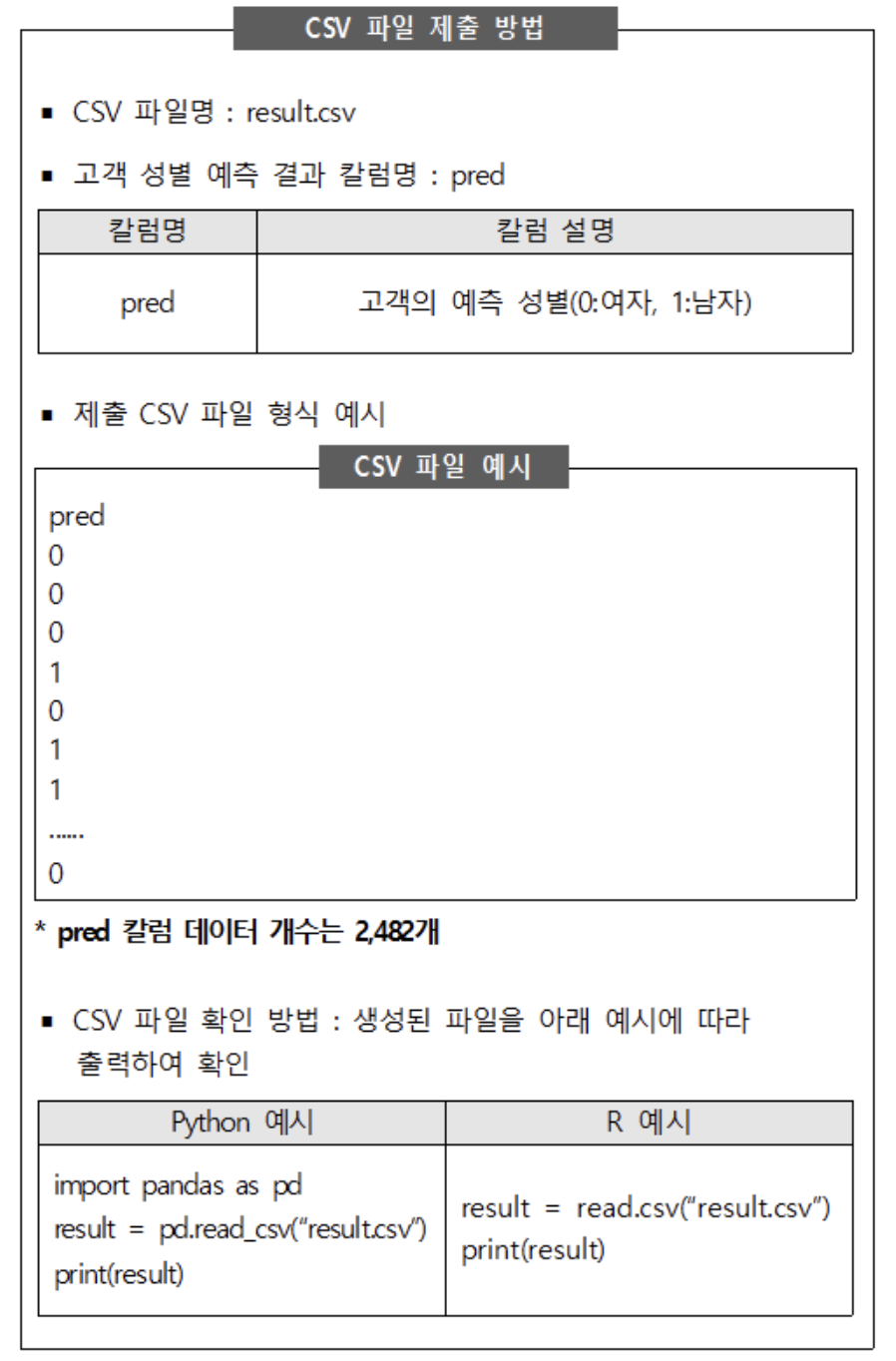
제공된 데이터는 백화점 고객이 1년간 상품을 구매한 속성 데이터이다. 제공된 학습용 데이터(data/customer_train.csv)를 이용하여 백화점 구매 고객의 성별을 예측하는 모델을 개발하고, 개발한 모델에 기반하여 평가용 데이터(data/customer_test.csv)에 적용하여 얻은 성별 예측 결과를 【제출 형식】에 따라 CSV 파일로 생성하여 제출하시오.

* 예측 결과는 ROC-AUC 평가지표에 따라 평가함

* 성능이 우수한 예측 모델을 구축하기 위해서는 데이터 정제, Feature Engineering, 하이퍼 파라미터(hyper parameter) 최적화, 모델 비교 등이 필요할 수 있음. 다만, 과적합에 유의하여야 함.

【제출 형식】

㉠ CSV 파일명 : result.csv (파일명에 디렉토리∙폴더 지정 불가)

㉡ 예측 성별 칼럼명 : pred

㉢ 제출 칼럼 개수 : pred 칼럼 1개

㉣ 평가용 데이터 개수와 예측 결과 데이터 개수 일치 : 2,482개

풀이 1. probit regression : 정확하지 않으므로 선호하지 않음

train = read.csv("./data/customer_train.csv")
test = read.csv("./data/customer_test.csv")
train = na.omit(train)
test = na.omit(test)

train$성별 = as.factor(train$성별)
model = glm(성별 ~ 총구매액 + 최대구매액 + 환불금액 + 방문일수 + 방문당구매건수 + 주말방문비율 + 구매주기,
					 data = train, family=binomial(link = 'probit'))
probabilities = predict(model, test)
pred = array()
for(i in 1:dim(test)[1]){
	pred[i] = as.numeric(probabilities[i] > 0.5)
}
pred = as.data.frame(pred) # to properly save a csv file

write.csv(pred, "result.csv", row.names = FALSE)
result = read.csv("result.csv")
print(result)

풀이 2. SVM

library(e1071)

train = read.csv("./data/customer_train.csv")
test = read.csv("./data/customer_test.csv")
train = na.omit(train)
test = na.omit(test)

train$성별 = as.factor(train$성별)
sv = svm(성별 ~ 총구매액 + 최대구매액 + 환불금액 + 방문일수 + 방문당구매건수 + 주말방문비율 + 구매주기,
					 data = train)
pred = predict(sv, test)
pred = as.data.frame(pred) # to properly save a csv file

write.csv(pred, "result.csv", row.names = FALSE)
result = read.csv("result.csv")
print(result)

풀이 3. 랜덤 포레스트 : SVM과 달리, 각 클래스별 확률을 계산할 수도 있음

library(randomForest)

train = read.csv("./data/customer_train.csv")
test = read.csv("./data/customer_test.csv")
train = na.omit(train)
test = na.omit(test)

train$성별 = as.factor(train$성별)
model = randomForest(성별 ~ 총구매액 + 최대구매액 + 환불금액 + 방문일수 + 방문당구매건수 + 주말방문비율 + 구매주기,
					 data = train)
pred = predict(model, test)
pred = as.data.frame(pred) # to properly save a csv file

write.csv(pred, "result.csv", row.names = FALSE)
result = read.csv("result.csv")
print(result)

예시 2. (정식 문제는 아님)

다음과 같은 예제 데이터가 주어져 있을 때, x_train, y_train으로부터 모델을 생성하여 x_test로부터 y_test를 예측하여라.

# Load required libraries
library(dplyr)
library(caret)

# Load the wine dataset
data(wine, package = "rattle")
wine_data <- wine

# Create a data frame for features (x) and target (y)
x <- wine_data %>% select(-Type)  # Select all columns except 'Type' which is the target
y <- wine_data %>% select(Type)   # Select only the 'Type' column

# Split the dataset into training and test sets
set.seed(123)  # For reproducibility
trainIndex <- createDataPartition(y$Type, p = 0.8, list = FALSE)
x_train <- x[trainIndex, ]
y_train <- y[trainIndex, ]
x_test <- x[-trainIndex, ]
y_test <- y[-trainIndex, ]

# Additional manipulations as per the Python code
x_test <- as.data.frame(x_test)
x_train <- as.data.frame(x_train)
y_train <- as.data.frame(y_train)

# Reset index in x_test (not typically done in R, but for parity with Python code)
x_test <- x_test %>% mutate(index = row_number()) %>% select(index, everything())

# Rename the column in y_train
names(y_train)[1] <- 'target'

풀이 1. SVM

library(e1071)

x_train['target'] = y_train[,1]
x_train$target = as.factor(x_train$target) # necessary
sv <- svm(target ~ ., data = x_train)
pred = predict(sv, x_test) 

print(sum(y_test == pred) / length(y_test)) # accuracy

풀이 2. 랜덤 포레스트 : SVM과 달리, 각 클래스별 확률을 계산할 수도 있음

library(randomForest)

x_train['target'] = y_train[,1]
x_train$target = as.factor(x_train$target) # necessary

model <- randomForest(target ~ ., data = x_train)
pred = predict(model, x_test)
print(sum(y_test == pred) / length(y_test)) # accuracy

prob_estimates <- predict(model, x_test, type = "prob") # SVM은 원리상 이 기능이 작동하지 않음

예시 3. (정식 문제는 아님)

다음과 같은 예제 데이터가 주어져 있을 때, x_train, y_train으로부터 모델을 생성하여 x_test로부터 y_test를 예측하여라.

# Load required libraries
library(dplyr)
library(caret)

# Load the iris dataset (included in base R)
data(iris)

# Rename the columns for consistency with the Python code
names(iris) <- c('sepal_length', 'sepal_width', 'petal_length', 'petal_width', 'species')

# Convert species to a binary factor: 'setosa' as 0 and others as 1
iris$species <- as.numeric(iris$species != 'setosa')

# Split the data into training and testing sets
set.seed(123)  # for reproducibility
trainIndex <- createDataPartition(iris$species, p = 0.8, list = FALSE)
trainData <- iris[trainIndex, ]
testData <- iris[-trainIndex, ]

# Convert first entry of sepal_length to NA (missing value)
trainData$sepal_length[1] <- NA
testData$sepal_length[1] <- NA

# Insert an outlier in sepal_width
trainData$sepal_width[1] <- 150

# Wrap-up
trainData = na.omit(trainData)
x_train = trainData[, 1:4]
y_train = trainData[5]
testData = na.omit(testData)
x_test = testData[, 1:4]
y_test = testData[, 5]

풀이 1. SVM

library(e1071)

x_train['species'] = y_train[,1]
x_train$species = as.factor(x_train$species) # necessary
sv <- svm(species ~ ., data = x_train)

pred = predict(sv, x_test)

print(sum(y_test == pred) / length(y_test)) # accuracy

풀이 2. 랜덤 포레스트 : SVM과 달리, 각 클래스별 확률을 계산할 수도 잇음

library(randomForest)

x_train['species'] = y_train[,1]
x_train$species = as.factor(x_train$species) # necessary

model <- randomForest(species ~ ., data = x_train)
pred = predict(model, x_test)
print(sum(y_test == pred) / length(y_test)) # accuracy

prob_estimates <- predict(model, x_test, type = "prob") # SVM은 원리상 이 기능이 작동하지 않음
prob_estimates

예시 4. (정식 문제는 아님)

다음과 같은 예제 데이터가 주어져 있을 때, x_train, y_train으로부터 모델을 생성하여 x_test로부터 y_test를 예측하여라.

# Load required libraries
library(tidyverse)
library(caret)

# Load the Titanic dataset from a package or a source that you have
# Note: Ensure that the dataset structure matches with what you expect
# For this example, I'm using the Titanic dataset from the datasets package
data("Titanic")
df <- as_tibble(Titanic)

# Selecting columns and target variable
# Adjust the column names according to your dataset
x <- select(df, -Survived) 
y <- df$Survived

# Split the data into training and test sets
set.seed(123) # for reproducibility
trainIndex <- createDataPartition(y, p = .8, list = FALSE, times = 1)
x_train <- x[trainIndex, ]
y_train <- y[trainIndex]
x_test  <- x[-trainIndex, ]
y_test  <- y[-trainIndex]

# Convert y_train and y_test to tibble with a new column name
y_train <- tibble(target = y_train)
y_train = as.data.frame(y_train)
y_test <- tibble(target = y_test)
y_test = as.data.frame(y_test)

# Convert x_train and x_test to tibble (optional if they are already tibbles)
x_train <- as_tibble(x_train)
x_train = as.data.frame(x_train)
x_test <- as_tibble(x_test)
x_test = as.data.frame(x_test)

풀이 1. SVM

library(e1071)

x_train['target'] = y_train
x_train$target = as.factor(x_train$target) # necessary

sv <- svm(target ~ ., data = x_train)
pred = predict(sv, x_test)
print(sum(y_test$target == pred) / length(y_test$target)) # accuracy

풀이 2. 랜덤 포레스트 : SVM과 달리, 각 클래스별 확률을 계산할 수도 있음

library(randomForest)

x_train['target'] = y_train
x_train$target = as.factor(x_train$target) # necessary

model <- randomForest(target ~ ., data = x_train)
pred = predict(model, x_test)
print(sum(y_test$target == pred) / length(y_test$target)) # accuracy
 
prob_estimates <- predict(model, x_test, type = "prob") # SVM은 원리상 이 기능이 작동하지 않음
prob_estimates

C. 3유형 (30점; 2문제; 문제마다 소문제 존재)

전략

필자의 경우 새로운 함수를 많이 익히지는 않는 방향으로 문제를 풀려고 함

예시 1.

제공된 데이터(data/Titanic.csv)는 타이타닉호의 침몰 사건에서 생존한 승객 및 사망한 승객의 정보를 포함한 자료이다. 아래 데이터를 이용하여 생존 여부(Survived)를 예측하고자 한다. 각 문항의 답을 【제출 형식】에 맞춰 답안 작성 페이지에 입력하시오. (단, 벌점화(penalty)는 부여하지 않는다.)

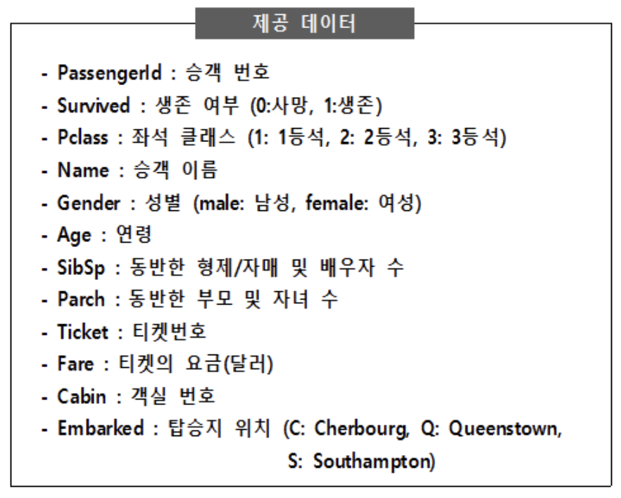
① Gender와 Survived 변수 간의 독립성 검정을 실시하였을 때, 카이제곱 통계량은? (반올림하여 소수 셋째 자리까지 계산)

② Gender, SibSp, Parch, Fare를 독립변수로 사용하여 로지스틱 회귀모형을 실시하였을 때, Parch 변수의 계수값은? (반올림하여 소수 셋째 자리까지 계산)

③ 위 ②번 문제에서 추정된 로지스틱 회귀모형에서 SibSp 변수가 한 단위 증가할 때 생존할 오즈비(Odds ratio) 값은? (반올림하여 소수 셋째 자리까지 계산)

【제출 형식】

㉠ 소수 넷째 자리에서 반올림하여 소수 셋째 자리까지만 계산

풀이.

① 카이제곱검정 테스트 : 답은 260.717

a <- read.csv("data/Titanic.csv")

library(dplyr)

result_chisq <- chisq.test(a$Gender, a$Survived)

print(round(result_chisq$statistic,3))

②, ③ 로지스틱 회귀 : 답은 각각 -0.201, 0.702

a <- read.csv("data/Titanic.csv")

# a = na.omit(a) : 관련 없는 칼럼에서 생긴 결측치를 가지고 튜플을 제외하면 최종답이 달라짐 

md_glm <- glm(Survived ~ Gender + SibSp + Parch + Fare, data=a, family=binomial(link="logit"))

val = as.numeric(md_glm[[1]][4])

print(round(val, 3))

val2 = as.numeric(md_glm[[1]][3])

print(round(exp(val2), 3))

입력: 2023.11.19 18:45

수정: 2023.11.22 13:10

저작자표시

'▶ 자연과학 > ▷ 컴퓨터과학' 카테고리의 다른 글

【빅데이터분석기사】 필기 키워드 정리 (0)	2023.11.19
【Excel】 Excel 단축키 모음 (0)	2021.09.09
【컴퓨터 활용】 Excel 목차 (0)	2018.10.05
【한글】 자주 쓰는 한글 단축키 (0)	2018.10.03
【컴퓨터 활용】 한글 자음 (ㄱ, ㄴ, ㄷ, ···) + 한자 및 기타 특수문자 (0)	2017.12.02

정빈이의 공부방

최근댓글

【빅데이터분석기사】 R 실기 필수 암기 및 예제

'▶ 자연과학 > ▷ 컴퓨터과학' 카테고리의 다른 글

티스토리툴바

【빅데이터분석기사】 R 실기 필수 암기 및 예제

'▶ 자연과학 > ▷ 컴퓨터과학' 카테고리의 다른 글

'▶ 자연과학/▷ 컴퓨터과학' 관련 포스팅

티스토리툴바