데이터 분석 : Kaplan-Meier 생존 곡선
추천글 : 【생물정보학】 생물정보학 분석 목차
1. 이번에 죽은 환자 수 [본문]
2. # of censored [본문]
3. 지금까지 살았을 확률 [본문]
4. R 코드 [본문]
5. 파이썬 코드 [본문]
| 총 걸린 시간 (t) | 이번에 죽은 환자 수 (d) | 전까지 살아있던 환자 수 (n) | # of censored | 이번에 죽었을 확률 (d/n) | 이번에 살았을 확률 (1 - d/n) | 지금까지 살았을 확률 (L) |
| 6 | 1 | 23 | 0 | 0.0435 | 0.9565 | 0.9565 |
| 12 | 1 | 22 | 0 | 0.0455 | 0.9545 | 0.9130 |
| 21 | 1 | 21 | 0 | 0.0476 | 0.9524 | 0.8695 |
| 27 | 1 | 20 | 0 | 0.0500 | 0.9500 | 0.8260 |
| 32 | 1 | 19 | 0 | 0.0526 | 0.9474 | 0.7826 |
| 39 | 1 | 18 | 0 | 0.0556 | 0.9444 | 0.7391 |
| 43 | 2 | 17 | 1 | 0.1176 | 0.8824 | 0.6522 |
| 89 | 1 | 14 | 5 | 0.0714 | 0.9286 | 0.6056 |
| 261 | 1 | 8 | 0 | 0.1250 | 0.8750 | 0.5299 |
| 263 | 1 | 7 | 0 | 0.1429 | 0.8571 | 0.4542 |
| 270 | 1 | 6 | 1 | 0.1667 | 0.8333 | 0.3785 |
| 311 | 1 | 4 | . | 0.2500 | 0.7500 | 0.2839 |
Table. 1. Kaplan-Meier 생존 곡선 예제
1. 이번에 죽은 환자 수(number of patients died) [목차]
⑴ 맨 첫 행의 23명의 경우, 시간이 0이었을 때 23명이 살아있었다는 의미
⑵ 두 번째 행의 22명의 경우, 시간이 6이었을 때 22명이 살아있었다는 의미
⑶ 이번에 살아있는 환자 수(number at risk)는 표시하기도 하고 안 하기도 함
2. # of censored [목차]
⑴ 환자가 더이상 입원을 하지 않는 등의 사정으로 더 이상의 기록이 존재하지 않는 것을 의미함
⑵ censored된 환자는 다른 생존한 환자들과 동일한 생존 확률을 가지고 있다고 가정
⑶ 일반적으로 그래프 상에서 ⊕으로 표시함
3. 지금까지 살았을 확률 [목차]
⑴ 시간 12까지 살았을 확률 = 0.9130 = 시간 6까지 살았을 확률 × 이번(6 ~ 12)에 살았을 확률 = 0.9565 × 0.9545
⑵ 시간 21까지 살았을 확률 = 0.8695 = 시간 12까지 살았을 확률 × 이번(12 ~ 21)에 살았을 확률 = 0.9130 × 0.9524
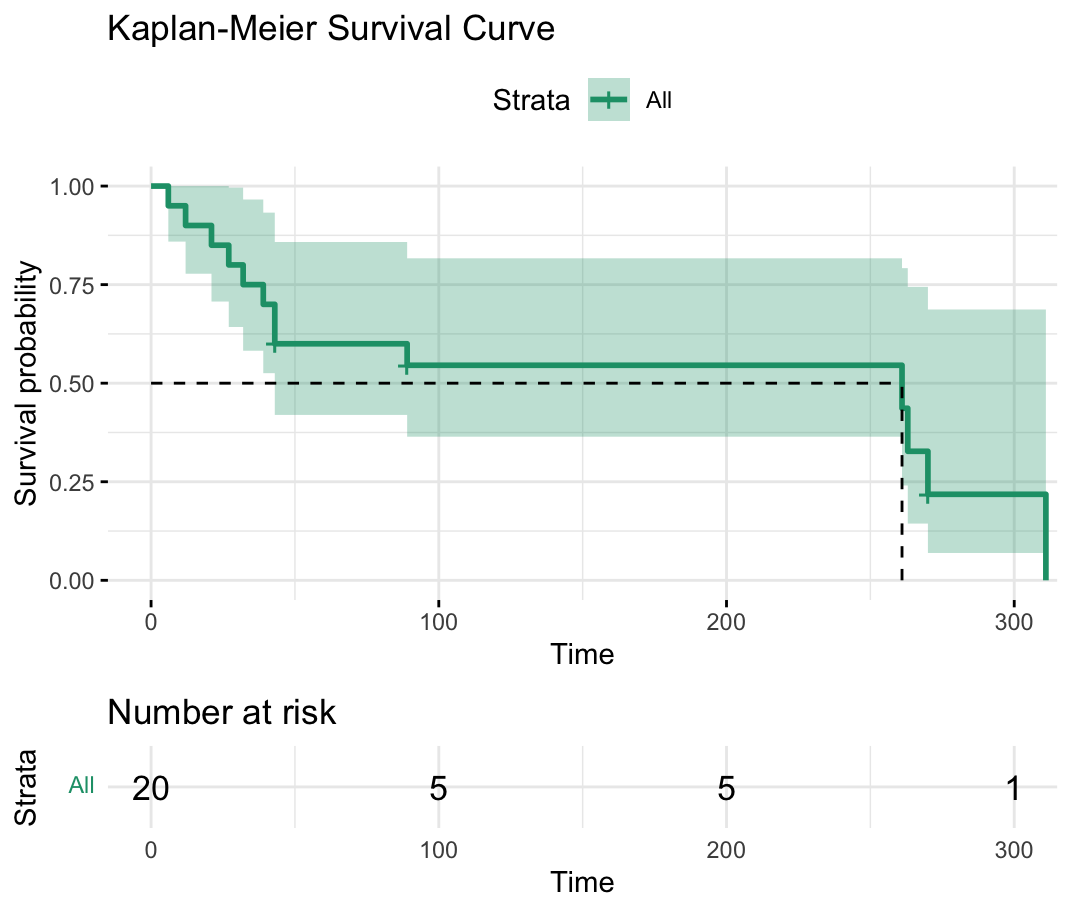
4. R 코드 [목차]
⑴ 생존곡선에 관한 R 코드 (단, # of censored 고려)
# 필요한 패키지 설치 및 로드
install.packages("survival")
install.packages("survminer")
library(survival)
library(survminer)

# 수정된 데이터 프레임 생성
# 모든 사망과 censoring 사건을 정확하게 반영
surv_data <- data.frame(
  time = c(6, 12, 21, 27, 32, 39, 43, 43, 43, 89, 89, 89, 89, 89, 89, 261, 263, 270, 270, 311),
  status = c(1, 1, 1, 1, 1, 1, 1, 1, 0, 1, 0, 0, 0, 0, 0, 1, 1, 1, 0, 1) # 사망은 1, censoring은 0
)

# Surv 객체 생성
surv_obj <- Surv(time = surv_data$time, event = surv_data$status)

# Kaplan-Meier 생존 곡선 추정
fit <- survfit(surv_obj ~ 1, data = surv_data)

# 생존 곡선 그리기
ggsurvplot(
  fit,
  data = surv_data,
  xlab = "Time",
  ylab = "Survival probability",
  title = "Kaplan-Meier Survival Curve",
  surv.median.line = "hv", # 중앙값 생존 시간 선 추가
  ggtheme = theme_minimal(), # 테마 설정
  risk.table = TRUE, # 위험 테이블 추가
  palette = "Dark2" # 색상 팔레트 설정
)
⑵ p-value를 추가한 경우 : 단, 다음 코드는 예시적 상황으로 위 표와 관련이 없음
library(survival)
library(survminer)

# Prepare Condition, Overall Survival Time, and Overall Survival Status
print(condition) # continuous variable
print(overall_surv_time)
print(overall_surv_status)

# Convert Overall Survival Status to a binary variable, where 1 = event occurred (DECEASED) and 0 = censored (LIVING or NA)
overall_surv_status_binary <- ifelse(overall_surv_status == "DECEASED", 1, 0)

# Create survival objects
surv_obj_overall <- Surv(time = overall_surv_time, event = overall_surv_status_binary)

# Find the median value of the condition
median_condition <- median(condition, na.rm = TRUE)

# Split data based on the median condition
data_overall <- data.frame(surv_obj_overall, Status = overall_surv_status_binary, Condition = condition)

# Overall Survival Analysis
ggsurvplot(
  survfit(surv_obj_overall ~ Condition >= median_condition, data = data_overall),
  data = data_overall,
  pval = TRUE,
  risk.table = TRUE,
  title = "Overall Survival based on Median Condition",
  legend.title = "Condition >= Median"
)
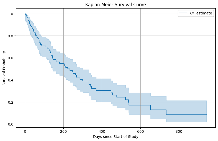
5. 파이썬 코드 [목차]
from lifelines import KaplanMeierFitter
import matplotlib.pyplot as plt
import pandas as pd
import numpy as np

# Simulate some survival data for demonstration purposes
np.random.seed(42)  # for reproducibility
n_patients = 100
study_duration = 1000  # days

# Generate some survival times with a predefined survival rate (we will use an exponential distribution)
survival_times = np.random.exponential(scale=365, size=n_patients)  # mean survival time

# Generate censoring times, assuming that if a patient hasn't had an event by the end of the study, they are censored
censoring_times = np.random.uniform(low=0, high=study_duration, size=n_patients)

# The observed time is the minimum of the survival time and censoring time
observed_times = np.minimum(survival_times, censoring_times)

# The event is observed if the survival time is less than or equal to the censoring time
events_observed = (survival_times <= censoring_times).astype(int)

# Create a DataFrame
df_patients = pd.DataFrame({
    'duration': observed_times,
    'event_observed': events_observed
})

# Fit the Kaplan-Meier survival estimator on the data
kmf = KaplanMeierFitter()
kmf.fit(df_patients['duration'], event_observed=df_patients['event_observed'])

# Plot the survival function
plt.figure(figsize=(10, 6))
kmf.plot_survival_function()
plt.title('Kaplan-Meier Survival Curve')
plt.xlabel('Days since Start of Study')
plt.ylabel('Survival Probability')
plt.grid(True)
plt.show()
입력: 2021.04.13 17:29
수정: 2024.03.11 21:42
'▶ 자연과학 > ▷ 생물정보학' 카테고리의 다른 글
| 【생물정보학】 RCTD의 이해 및 실행 (0) | 2021.06.03 |
|---|---|
| 【생물정보학】 CellPhoneDB의 이해 (0) | 2021.04.13 |
| 【생물정보학】 MIA 분석의 이해 및 실행 (0) | 2021.01.02 |
| 【생물정보학】 scater로 cell type 결정하기 (0) | 2019.12.20 |
| 【생물정보학】 Seurat로 cell type 결정하기 (7) | 2019.11.25 |


최근댓글